Working with Time Series in MDX Views

In this part we will look at using some of the Time Series functions allowing us to create views with Year-on-Year comparisons, rolling averages, moving sums etc.

Configure Level Names

Level names give you the ability to reference levels within a hierarchy by a more meaningful name e.g. Month, Quarter, Half or Year, rather than level000, level 001 etc.

Configuring level names is still very limited. Where multiple rollups exist in the same hierarchy, you can only apply one set of naming e.g. Month, Quarter, Half and Year if that is how your period dimension is structured. Essentially this means that Month is always the leaf level and Quarters are the parent.

If you have another rollup that is simply Month into Year, selecting a named level like Quarter will actually return years. This also depends on the basis of your set but hopefully the example is simple enough.

Keep in mind that you can create an alternate hierarchy should you wish to keep to single rollups in each hierarchy.

Update }HierarchyProperties

To name the level, there are two options:

Recent changes in the PAW dimension editor allow you to update the naming directly. You can access the names by clicking on the kebab menu next to the hierarchy then selecting Customize level names.

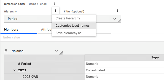
The following window displays allowing updates to the level names.

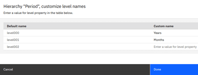
Once updated and you click Done, the level naming is applied and available for use in sets.

The legacy option requires a few more steps as well as a process to refresh the hierarchy.

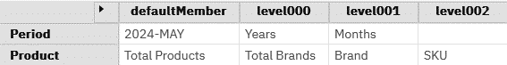
In my example I will keep it simple and have Years and Months for Period and then use my Brands rollup for Product.

Open the }HierarchyProperties cube from the Control Objects then type in the relevant names. In my example I will keep it simple and have Years and Months for Period and the use my Brands rollup for Product.

Refreshing the MDX Hierarchies

If updating using the legacy approach, you will need to run a process to refresh the hierarchies affected.

My process has the following in the Prolog:

				
					RefreshMdxHierarchy( 'Period' );
RefreshMdxHierarchy( 'Product' );

You could also run do the following to refresh all dimensions:

				
					RefreshMdxHierarchy( '' );

Reviewing the Level Names

We can run some MDX against our }ElementAttributes_Period cube to show the effect of our changes:

				
					WITH 
MEMBER [}ElementAttributes_Period].[}ElementAttributes_Period].[Level] AS 
	[Period].[Period].CURRENTMEMBER.LEVEL.ORDINAL
MEMBER [}ElementAttributes_Period].[}ElementAttributes_Period].[Level Name] AS 
	[Period].[Period].CURRENTMEMBER.LEVEL.NAME	
	
SELECT 
{[}ElementAttributes_Period].[}ElementAttributes_Period].[Level], [}ElementAttributes_Period].[}ElementAttributes_Period].[Level Name]} ON 0,
{TM1SubsetToSet([Period].[Period],"Default","public")} ON 1 
FROM [}ElementAttributes_Period]

The above code will give us two columns, one with the level number and another with the level name.

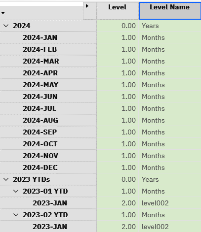
From the above view, you can see that the changes have applied but unfortunately where we have a rollup like the Year-to-Date (YTDs), there is an additional level which confuses the naming. Be aware of this when you have multiple rollups.

Also keep in mind that Level 0 are root entries, their children are Level 1 etc. Some TM1 functions like ELLEV() or ElementLevel() start with Level 0 being the leaf elements then work up to the root elements. Root elements which are marked as Level 0 in the above would in TM1 functions be a mixture of 1’s and 2’s. Be aware of this difference so that you can handle these accordingly, especially with ragged hierarchies.

Similarly for Product we could execute a similar set of MDX to show us the configured levels:

				
					WITH 
MEMBER [}ElementAttributes_Product].[}ElementAttributes_Product].[Level] AS 
	[Product].[Product].CURRENTMEMBER.LEVEL.ORDINAL
MEMBER [}ElementAttributes_Product].[}ElementAttributes_Product].[Level Name] AS 
	[Product].[Product].CURRENTMEMBER.LEVEL.NAME	
	
SELECT 
{[}ElementAttributes_Product].[}ElementAttributes_Product].[Level], [}ElementAttributes_Product].[}ElementAttributes_Product].[Level Name]} ON 0,
{TM1SubsetToSet([Product].[Product],"Default","public")} ON 1 
FROM [}ElementAttributes_Product]

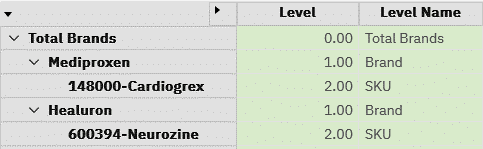
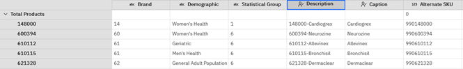
Expanding the Total Brands rollup and the Brands, we can see the levels and level names we configured.

So where does all this get us then? In various functions we need to specify a level on which to base a lookup e.g. on ParallelPeriods()

				
					Syntax: PARALLELPERIOD(level expression , lag , member)

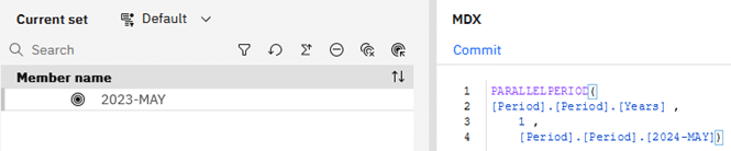
If we want last year, we need to specify the level reference as Year so that we lookup relative to Years and not Months.

				
					PARALLELPERIOD([Period].[Period].[Years] , 
1 ,
[Period].[Period].[2024-MAY])

ParallelPeriod() always returns a member from a prior period and is thus useful for our Year-on-Year (YoY) view.

Similarly, if we used the Months level instead of Years we would have returned the prior Month:

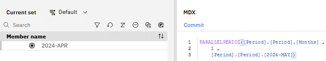
Worth noting too is that using a negative index would return a future period e.g. 2025-MAY in the first example and 2024-JUN in the second example.

Year-on-Year View

				
					WITH 
	MEMBER [Sales Measures].[Sales Measures].[PY] AS
	([Sales Measures].[Sales Measures].[Units],
		ParallelPeriod([Period].[Period].[Years],
		1,
		[Period].[Period].CurrentMember)
	),
	FORMAT_STRING = "#,##0;-#,##0;"
	
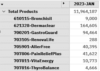
SELECT {[Sales Measures].[Sales Measures].[Units], [Sales Measures].[Sales Measures].[PY]} ON 0, 
NON EMPTY {Descendants([Product].[Product].[Total Products])} ON 1 
FROM [Sales] 
WHERE ([Scenario].[Scenario].[Actual], [Period].[Period].[2024-JAN], [Customer].[Customer].[Total Customers])

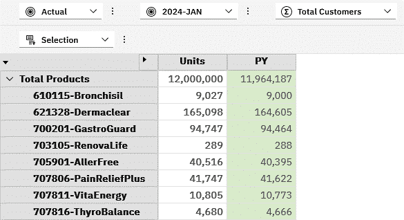
Unfortunately, the Caption property for calculated members is not currently recognized in PAW otherwise we could have built a string and assigned it to the Caption of PY e.g. PY-2023-JAN

For now, the reader will just need to interpret what PY means in relation to the selected Period.

If we create another view manually in PAW to verify the numbers being displayed in the PY, they align correctly with our previous view:

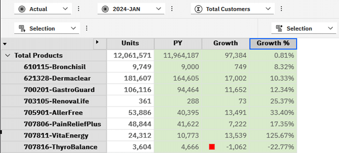
Using some of what we have learned previously we can now add a measure for Growth and Growth % and get some insights into what we are reading:

				
					WITH 
	MEMBER [Sales Measures].[Sales Measures].[PY] AS
	([Sales Measures].[Sales Measures].[Units],
		ParallelPeriod([Period].[Period].[Years],
		1,
		[Period].[Period].CurrentMember)
	),
	SOLVE_ORDER=1, FORMAT_STRING = "#,##0;-#,##0;"
	
	MEMBER [Sales Measures].[Sales Measures].[Growth] AS
		[Sales Measures].[Sales Measures].[Units] - [Sales Measures].[Sales Measures].[PY],
	SOLVE_ORDER=2, FORMAT_STRING = "#,##0;-#,##0;"
	
	MEMBER [Sales Measures].[Sales Measures].[Growth %] AS
	IIF(
		[Sales Measures].[Sales Measures].[PY] = 0,
		0,
		[Sales Measures].[Sales Measures].[Growth] / [Sales Measures].[Sales Measures].[PY]
		),
	SOLVE_ORDER=3, FORMAT_STRING = "0.00%;-0.00%"
	
SELECT {[Sales Measures].[Sales Measures].[Units], [Sales Measures].[Sales Measures].[PY], 
	[Sales Measures].[Sales Measures].[Growth], [Sales Measures].[Sales Measures].[Growth %]} ON 0, 
NON EMPTY {Descendants([Product].[Product].[Total Products])} ON 1 
FROM [Sales] 
WHERE ([Scenario].[Scenario].[Actual], 
[Period].[Period].[2024-JAN], 
[Customer].[Customer].[Total Customers])

I made use of the SOLVE_ORDER to ensure that we derive the measures in the correct order by explicitly setting these. They are not always required but probably a good habit to follow.

I also included an IIF() function to trap any divide by zero cases and handle them.

I also selected the Growth column and using the Format Manager added a conditional rule to the column highlighting where Growth is negative. The resultant view is below:

Set Basics

Before we can look at using some of the Time Series functions further, we need to understand some of the limitations we will face in trying to add the Period and other members relating to that Period.

The first thing we need to be able to do is to determine the base Period or reference Period to be used in the view.

It would be intuitive to have the Period on the Context/Slicers so that you could select a different value and then have your MDX update based on the selection.

Unfortunately this translates into having the same dimension on multiple axes and does not work.

The simplest option for now is to use a Period from a set, like the Current Period set. Another slightly more complicated solution which we will look at in the future is using a user preferences cube where users could update a period using a picklist and that is then used as the basis for the MDX.

Using MDX to return the member from our Current Period set, we would have some code like the following:

				
					SELECT 
NON EMPTY {TM1SubsetToSet([Period].[Period],"Current Period", "public")} *
	{[Sales Measures].[Sales Measures].[Units]} ON 0, 
NON EMPTY {TM1SubsetToSet([Product].[Product],"All Products", "public")} ON 1 
FROM [Sales] WHERE (
	[Scenario].[Scenario].[Actual], 
	[Customer].[Customer].[Total Customers])

Our view would be returned as follows:

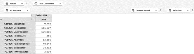
Note that the TM1SubsetToSet() function has the third argument to tell it to use either a pubic or private set. Where you have something like Current Period it may be that you have both and would be something to watch out for.

From the above query, we can extend this a bit further by adding a new function to allow us to reference Calculated Sets. A Calculated Set like a Calculated Member is derived at time of execution based on the underlying references at that point in time.

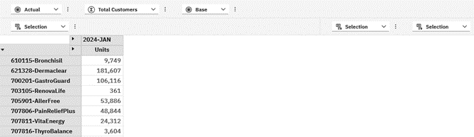
As a simple example, let’s move the TM1SubsetToSet() into a Calculated Set:

				
					WITH
SET [Periods] AS {TM1SubsetToSet([Period].[Period],"Current Period", "public")}

SELECT 
NON EMPTY {[Periods]} *
	{[Sales Measures].[Sales Measures].[Units]} ON 0, 
NON EMPTY {TM1SubsetToSet([Product].[Product],"All Products", "public")} ON 1 
FROM [Sales] WHERE (
	[Scenario].[Scenario].[Actual], 
	[Customer].[Customer].[Total Customers])

I updated the conditional formatting too and now have something like this where the issue is clearly highlighted:

The results are identical, however you will notice that PAW is now showing Selection where previously it had the named of the Set selected. Using the Set editor will not return anything useful other than the standard sets as the members are now derived based on what was specified in the Calculated Set.

Let’s extend the previous query by firstly creating a Calculated Member with the current period and then using that to create our Calculated Set.

				
					WITH 
MEMBER [Period].[Period].[CP] AS 
	TM1SubsetToSet([Period].[Period],"Current Period", "public").Item(0).Item(0)
SET [Periods] AS
	{[Period].[Period].[CP]}

SELECT 
NON EMPTY {[Periods]} *
	{[Sales Measures].[Sales Measures].[Units]} ON 0, 
NON EMPTY {TM1SubsetToSet([Product].[Product],"All Products","public")} ON 1 
FROM [Sales] WHERE (
	[Scenario].[Scenario].[Actual], 
	[Customer].[Customer].[Total Customers])

Let’s assume that for some purpose we need to concatenate our Demographic and Caption using a vertical pipe separator into a Key e.g. Women’s Health|Cardiogrex for Product 148000. Let’s assume too that this is only relevant on Leaf members again.

Our adjusted code would simply use the + (plus) operator to join the three strings together:

Executing the MDX gives us the following view:

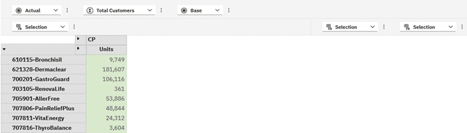
A few things to notice in the above results:

CP was used as the name of the Calculated Member. Using the same name as an existing set results in an error. You could call this anything else that makes sense in the context of your model though. For now we will read CP as Current Period when interpreting the results.

Note too that the CP/Units column is now green showing that it is derived.

A more subtle but very important component of the MDX is the way I dealt with the TM1SubsetToSet() function.

				
					TM1SubsetToSet([Period].[Period],"Current Period", "public").Item(0).Item(0)

Assuming the Current Year is 2024 and the Current Year Periods is based on this, I would expect the above to return to 2024-APR, the fourth element based on a zero index.

If we come back up the rabbit-hole, where does all of the above get us?

We can retrieve a member based on a set which when refreshed, would reflect the current member in that set and hence the view would be based on that member, the current period in this case.

We also used it as the basis for our new Calculated Set and this is really where we needed to be to leverage some of the other Time Series functions.

Last n Months

We can now use the above code and expand it to give us some more insights into the last 6 months for example.

The Last Periods function takes two parameters: The number of periods and the member in question.

				
					Syntax: LastPeriods(count, member)

Applying this to our code we can include the 6 periods and our CP member.

				
					WITH 
SET [CP] AS 
	{TM1SubsetToSet([Period].[Period],"Current Period", "public").Item(0).Item(0)}
SET [Periods] AS
	{LastPeriods(6,[CP].Item(0).Item(0))}

SELECT 
NON EMPTY {[Periods]} *
	{[Sales Measures].[Sales Measures].[Units]} ON 0, 
NON EMPTY {TM1SubsetToSet([Product].[Product],"All Products","public")} ON 1 
FROM [Sales] WHERE (
	[Scenario].[Scenario].[Actual], 
	[Customer].[Customer].[Total Customers])

I have added another set based on the CP, current period. Using a combination of the current period and the LastPeriods() function, we can get a dynamic 6 month view. When we update the member in the Current Period set, our view would update accordingly.

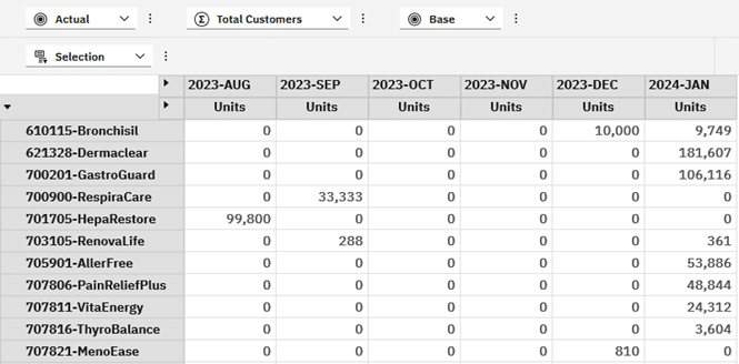
In my case I get the following view where 2024-JAN is my current period:

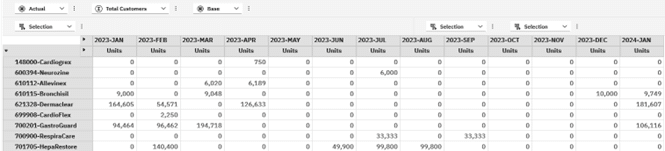
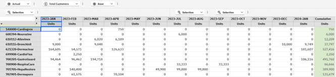
Similarly, if I had specified 13 periods to give a view of the same month in the prior year, I would have the following:

I could then extend this further by adding a Calculated Member to give me the sum across the periods.

				
					WITH 
MEMBER [Period].[Period].[Cumulative] AS
	SUM([Periods])
SET [CP] AS 
	{TM1SubsetToSet([Period].[Period],"Current Period", "public").Item(0).Item(0)}
SET [Periods] AS
	{LastPeriods(6,[CP].Item(0).Item(0))}

SELECT 
NON EMPTY {[Periods], [Period].[Period].[Cumulative]} *
	{[Sales Measures].[Sales Measures].[Units]} ON 0, 
NON EMPTY {TM1SubsetToSet([Product].[Product],"All Products","public")} ON 1 
FROM [Sales] WHERE (
	[Scenario].[Scenario].[Actual], 
	[Customer].[Customer].[Total Customers])

The extra column would be added and show the cumulative value:

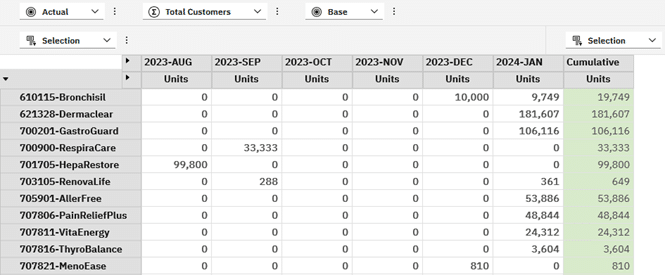
And likewise where we had 13 periods specified:

Going back to Part 3 of this series, you could likewise use AVG(), MIN(), MAX() etc. across the Periods set to give you additional insights.

Next n Months

This would typically be more useful when looking at your forecast or planning periods. There is no NextPeriods() function but we can combine what we have learned about ParallelPeriod() and LastPeriods() to give us a view of the future.

If we wanted a view of the next 6 months, including the current period, we could do the following:

				
					WITH 
SET [CP] AS 
	{TM1SubsetToSet([Period].[Period],"Current Period", "public").Item(0).Item(0)}
SET [Periods] AS
	LastPeriods(
		6,
		ParallelPeriod(
				[Period].[Period].[Months], 
				-5, 
				[CP].Item(0).Item(0)
			)
		)
SELECT 
{[Periods]} *
	{[Sales Measures].[Sales Measures].[Units]} ON 0, 
NON EMPTY {TM1SubsetToSet([Product].[Product],"All Products","public")} ON 1 
FROM [Sales] WHERE (
[Scenario].[Scenario].[Rolling Forecast], 
	[Customer].[Customer].[Total Customers])

Note that in the ParallelPeriod() function we are using a negative number to go forward in time and using 5 periods so that when we use LastPeriods() with a value of 6 the current period is included.

The period related MDX can be reduced further using a negative index against LastPeriods()

				
					WITH 
SET [CP] AS 
	{TM1SubsetToSet([Period].[Period],"Current Period", "public").Item(0).Item(0)}
SET [Periods] AS 
LastPeriods(-6,[CP].Item(0).Item(0))
SELECT 
{[Periods]} *
	{[Sales Measures].[Sales Measures].[Units]} ON 0, 
NON EMPTY {TM1SubsetToSet([Product].[Product],"All Products","public")} ON 1 
FROM [Sales] WHERE (
[Scenario].[Scenario].[Rolling Forecast], 
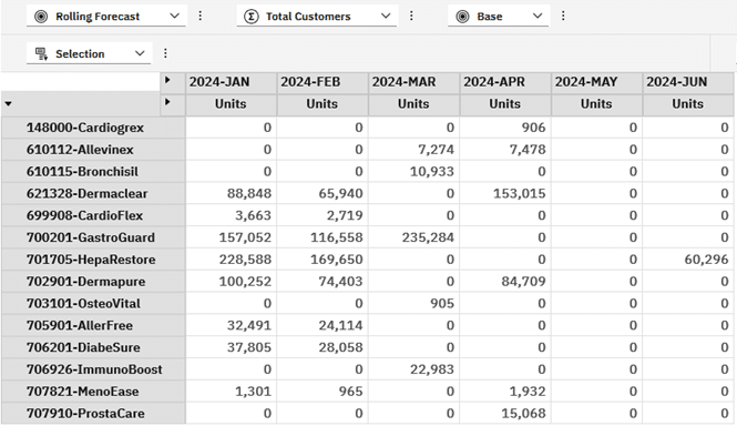
	[Customer].[Customer].[Total Customers])

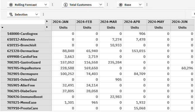
I also removed the NON EMPTY on columns to include 2024-MAY which has no planned values.

Periods To Date

We can use the PeriodsToDate() function to give use all the members based on the preceding siblings of the current member.

				
					Syntax: PeriodsToDate(level_expression, member)

The level_expression needs to be supplied as a higher level than the member so that there is a consolidation on which to base the sibling periods. In our example we are going to specify our Years level so that we return the sibling periods in the same year as our member.

We will also change the basis for our view from Actual to the Rolling Forecast and our Current Period set for our period to a different set with a future period to give a better view of what this function returns.

Our period set, Planning Period, is set to 2024-JUN i.e. the 6^th month in our fiscal year.

				
					WITH 
SET [CP] AS 
	{TM1SubsetToSet([Period].[Period],"Planning Period", "public").Item(0).Item(0)}
SET [Periods] AS
	{PeriodsToDate([Period].[Period].[Years], [CP].Item(0).Item(0))}

SELECT 
{[Periods]} *
	{[Sales Measures].[Sales Measures].[Units]} ON 0, 
NON EMPTY {TM1SubsetToSet([Product].[Product],"All Products","public")} ON 1 
FROM [Sales] WHERE (
	[Scenario].[Scenario].[Rolling Forecast], 
	[Customer].[Customer].[Total Customers])

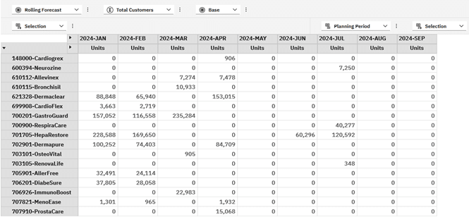
With this code, we get the following view returned:

And similarly if we were to change our planning period to 2024-SEP:

Opening Period

Maybe not that useful in a sales related example but more relevant to a balance sheet example where you would want to compare the current period to an opening period to understand the movement over time.

We will however explore the concept on sales to keep the examples aligned to previous examples.

With the OpeningPeriod() function we essentially are retrieving the first child in a given level/consolidation. Where we are looking at a planning period of 2024-SEP per our last example, we would expect the opening periods to be 2024-JAN based on our Period dimension that is configured as January to December each year.

				
					WITH 
SET [CP] AS 
	{TM1SubsetToSet([Period].[Period],"Planning Period", "public").Item(0).Item(0)}
SET [Periods] AS
	{OpeningPeriod([Period].[Period].[Months], [CP].Item(0).Item(0).Parent)}

SELECT 
{[Periods]} *
	{[Sales Measures].[Sales Measures].[Units]} ON 0, 
NON EMPTY {TM1SubsetToSet([Product].[Product],"All Products","public")} ON 1 
FROM [Sales] WHERE (
	[Scenario].[Scenario].[Rolling Forecast], 
	[Customer].[Customer].[Total Customers])

As expected, we are seeing values for 2024-JAN.

We could expand this code now to give us the Opening Period, Planning Period and a Variance.

				
					WITH 
MEMBER [Period].[Period].[Variance] AS
	([CP].Item(0) - [Periods].Item(0))
SET [CP] AS 
	{TM1SubsetToSet([Period].[Period],"Planning Period", "public").Item(0).Item(0)}
SET [Periods] AS
	{OpeningPeriod([Period].[Period].[Months], [CP].Item(0).Item(0).Parent)}
SELECT 
{[Periods], [CP], [Period].[Period].[Variance]} *
	{[Sales Measures].[Sales Measures].[Units]} ON 0, 
NON EMPTY {TM1SubsetToSet([Product].[Product],"All Products","public")} ON 1 
FROM [Sales] WHERE (
	[Scenario].[Scenario].[Rolling Forecast], 
	[Customer].[Customer].[Total Customers])

In the above MDX, we create a new Calculated Member called Variance to give us the variance or growth, depending on your interpretation. Remember that our members are actually sets and we first need to retrieve the member from the set before we can do the calculation.

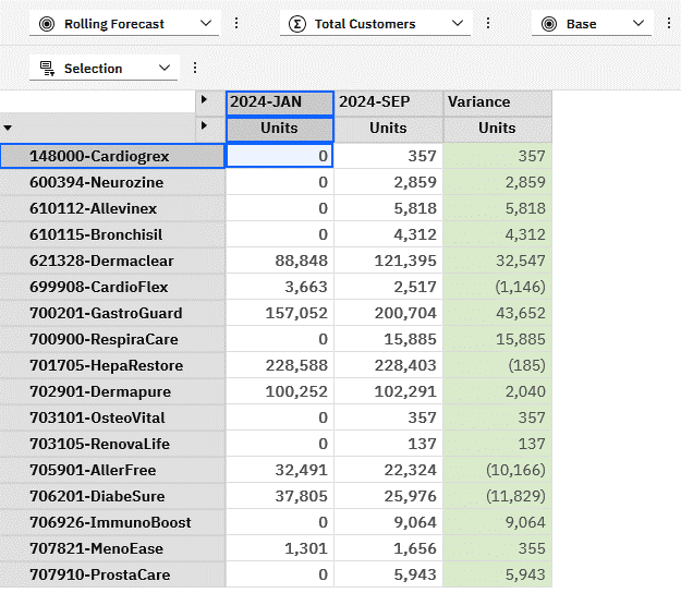
The resultant view is thus as follows:

Closing Period

As you probably guessed, this would give us the last period in a given level/consolidation and in our example this would be 2024-DEC. This may not seem that useful but can be useful to show use the remaining periods and a cumulative total which may be used in phasing to achieve our targets.

We will combine a couple of concepts from previous examples to get this view working.

For our Periods that will be shown, we would want to show from the current Planning Period to the end of the year. To achieve this we will overlay two sets of PeriodsToDate and remove the overlap i.e. prior periods before our planning period. With only the relevant periods, we can show these along with a cumulative result.

				
					WITH 
MEMBER [Period].[Period].[Cumulative] AS
	SUM([Periods])
	
SET [CP] AS 
	{TM1SubsetToSet([Period].[Period],"Planning Period", "public").Item(0).Item(0)}
SET [Periods] AS
		{ Except(
			PeriodsToDate([Period].[Period].[Years],
				ClosingPeriod([Period].[Period].[Months], [CP].Item(0).Item(0).Parent)
				),
			PeriodsToDate([Period].[Period].[Years], [CP].Item(0).Item(0).Lag(1))
			)}
	
SELECT 
{[Periods], [Period].[Period].[Cumulative]} *
	{[Sales Measures].[Sales Measures].[Units]} ON 0, 
NON EMPTY {TM1SubsetToSet([Product].[Product],"All Products","public")} ON 1 
FROM [Sales] WHERE (
	[Scenario].[Scenario].[Rolling Forecast], 
	[Customer].[Customer].[Total Customers])

Note: You could use the colon syntax to give you a range between members but this will require some changes to the above code and may, in some other cases include unwanted members depending on the structure of your dimension.

Note too that we added a Lag(1) to the current period to ensure that it is included in the view and totals. Depending on your use case, you may choose to include or exclude and may need to deal with period 1 i.e. January differently. Using Lead(n) would return a member n positions after the current member.

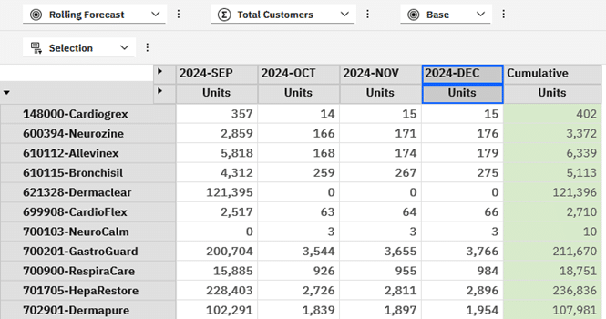
The resultant view is giving us exactly what we need to see the remaining periods as well as a cumulative total that i.e. our target in the planning periods:

In many models YTG rollups are typically created and could be leveraged in the MDX making your code even easier. If you do not have these rollups then using the above may be more practical than adding additional rollups to your model.

Applying Averages

In Part 3 we looked at the AVG() function. This will return the average across non-empty periods in our example i.e. a monthly average where there were sales recorded, rather than the monthly average of sales for the period. Both averages are typically used across models but for different purposes.

To illustrate the differences, the MDX code below gives a view of both as well as the cumulative values and a count of periods with sales.

				
					WITH 
MEMBER [Period].[Period].[Cumulative] AS
	SUM([Periods])
MEMBER [Period].[Period].[PeriodsMeasured] AS
	COUNT(
		FILTER(
			[Periods],
			[SalesMeasures].[Sales Measures].[Units] > 0
			)
		)
MEMBER [Period].[Period].[PeriodAvg] AS
		AVG([Periods])
MEMBER [Period].[Period].[PeriodAverage] AS
		[Period].[Period].[Cumulative] / 
		COUNT( [Periods] )
SET [CP] AS 
	{TM1SubsetToSet([Period].[Period],"Current Period", "public").Item(0).Item(0)}
SET [Periods] AS
	{LastPeriods(6,[CP].Item(0).Item(0))}

SELECT 
NON EMPTY {[Periods], [Period].[Period].[PeriodAverage], [Period].[Period].[Cumulative], 
	[Period].[Period].[PeriodsMeasured], [Period].[Period].[PeriodAvg]} *
	{[Sales Measures].[Sales Measures].[Units]} ON 0, 
NON EMPTY {TM1SubsetToSet([Product].[Product],"All Products","public")} ON 1 
FROM [Sales] WHERE (
	[Scenario].[Scenario].[Actual], 
	[Customer].[Customer].[Total Customers])

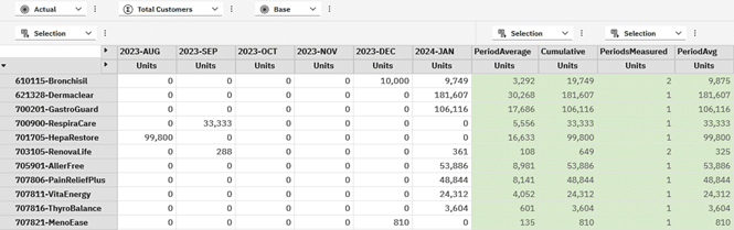
The view now gives us the average over the 6 months, the cumulative total, the count of periods with sales and the average sold in periods with sales.

As an exercise, something that is often required is a view showing a variance to budget or forecast and where we are behind target, phasing of the difference is needed to ensure that in future months we consider the sales to be caught up to achieve target. Are you able to add the variance and sum of year-to-go etc. to give you these insights?

Summary

In this part we started off by looking at how to name our levels so that we could address levels in the dimension and use these to get the members we needed e.g. siblings.

We then looked at some examples to get a year-on-year view by using ParallelPeriod() and extended this to give a view of growth and growth %.

Set basics covered some topics needed for the later examples where we use members from a specific set to drive the views we are using as part of our analysis.

Using the Current Period set, we looked at examples using syntax to get related periods based on LastPeriods(), combined this with ParallelPeriod() to get a forward looking view and added some code to sum the periods to show a sum and average across our timeline.

Extending these concepts further, PeriodsToDate() was introduced to look at a set of periods up to the current period i.e. a dynamic Year-To-Date view.

OpeningPeriod() and ClosingPeriod() were also introduced to look at examples where a starting point and movement over time is of relevance.

Lastly, some examples of averaging were reviewed with a focus on the distinction between showing an arithmetic mean where all periods were included whether they had a value or not, versus the weighted average that the AVG() function provides where only non-zero periods are included.

In the next part we will look at extending what we have learned here by introducing User Preferences which can act as the basis for the underlying queries rather than using a set like Current Period.

A summary of the MDX view related keywords used up to now:

Keyword	Description

Select	Specifies that you are looking to retrieve data from the cube
Non Empty	Removes all empty tuples from the specified set combinations on each axis. NON EMPTY can be used with both SELECT and ON clauses to filter axes or sets, not just “set combinations.”
On	Allows you to specify the relevant axis
From	Specifies the underlying cube to retrieve the data from
Where	Filters the query or view based on the specified tuple. This is an oversimplification and may require additional reading as it behaves more like a global filter.
With	Tells the MDX to define a temporary calculated member or measure which lasts for the duration of the MDX query. It can also be used to define sets. WITH, MEMBER and AS are typically found together when working with calculated members.
Member	This defines the context and name of the calculated member as part of the WITH clause. Multiple Member statements can be added to the MDX to create additional calculated members.
As	Just a declarative almost like saying Let var = x and tells MDX to assign the calculation to the member
Solve_Order	Where queries are complex and there are dependencies between calculated members, you will need to consider using the solve order to prevent sequencing or logical errors, ensuring correct evaluation.
Format_String	Allows the calculated member to be formatted for presentation to the user. These could be numerical formats similar to what you have used in Excel, currency, dates, and conditional formatting to show formats for positive, negative and zero values.
Sum	Calculates the total of a numeric expression evaluated over a set.
Aggregate	Aggregates a set of tuples by applying the appropriate aggregation function, like sum or count, based on the context.
Min	Finds the minimum value of a numeric expression evaluated over a set.
Max	Finds the maximum value of a numeric expression evaluated over a set.
Stdev	Computes the standard deviation of a numeric expression over a set, measuring the amount of variation or dispersion of the set.
Var	Calculates the variance of a numeric expression evaluated over a set, indicating how spread out the numbers are.
IIF()	The Immediate IF statement allows us to evaluate an expression for a certain condition and the return a result if true and a different result if false.
Case, When, Else, End	The Case statement would be used where you expect multiple outcomes or need to extend the conditions beyond true and false. The first WHEN statement that returns true is returned as the result. An ELSE can be used for a catch-all scenario or default result.
.CurrentMember	Allows us to address the current member the view is dealing with from the context area or another axis.
.Properties(“<propertyname>”<, TYPED>)	Allows us to retrieve a property value which may be an intrinsic like the Element_Level or custom like an attribute that a modeller added. Using TYPED ensures that a data type relating to the underlying definition is returned.
Instr()	Returns the position of a substring within a string, similar to TI’s Scan()
Len()	Returns the length of a string
Left()	Returns the n number of characters from the start of a string
Right()	Returns the n number of characters from the end of a string
LCase()	Returns the lower case of a string
UCase()	Return the upper case of a string
ParallelPeriod()	Returns a member from a prior period in the same relative position within a parallel period e.g. same month, last year.
LastPeriods()	Returns a set of members starting from the specified member and going backwards through the hierarchy by a specified number of periods. If given a negative number, it moves forward through the hierarchy.
PeriodsToDate()	Returns a set of periods from the beginning of a specified level to the specified member. Typically used with year-to-date views as YTD() is not supported by TM1.
OpeningPeriod()	Returns the first member of a specified level within a specified period or its ancestor e.g. January as the first month in our year.
ClosingPeriod()	Returns the last member of a specified level within a specified period or its ancestor e.g. December as the last month in our year.
Lag()	Returns the member that is a specified number of periods before the specified member in the same level. The lag can be positive to move backwards or negative to move forwards.
Lead()	Returns the member that is a specified number of periods after the current member in the same level. Similar to Lag(), you can switch signage to move backwards but better to use Lag() and Lead() as designed for better readability.

Special thanks to Wim Gielis for providing additional insights and proof-reading.

By George Tonkin, Business Partner at MCi.