Learning MDX Views in IBM Planning Analytics - Part 3

Aggregate Calculated Members in MDX

In Part 2, we introduced Calculated Members and looked the syntax needed to add these into our MDX code. We focused on arithmetic calculations that derived new members based on an existing sales measure. Our Calculated Members VAT and Sales Revenue incl VAT were derived from Sales Revenue, VAT by multiplying out the Sales Revenue by 15% and Sales Revenue incl VAT by adding Sales Revenue and VAT together.

That is great for the use case but what happens where you have multiple or hundreds of members and need to get the sum or aggregate value of these. Adding a calculated member and trying to specify each underlying member to be added together would be impractical, especially if these members change over time.

In TM1 Architect and Perspectives, when a user viewed a cube and needed to sum of the values across two or more members in a dimension, they could highlight the members and then click on the Rollup button to the right of the set editor.

This would create a custom rollup that was private to the user and could not be viewed by other users but allowed the user to see a total and the value of the members within that total.

PAW and Planning Analytics for Excel (PAfE) do not have this ability when viewing data in a cube view and working with members in the set editor.

There is however a way to perform this function in PAW and PAfE through MDX which gives far more flexibility in terms of the functions that can be applied as well as the ability for all users to see these totals.

PAfE also offers the TM1Set function where you could apply the concepts below to a set, but that is for another article.

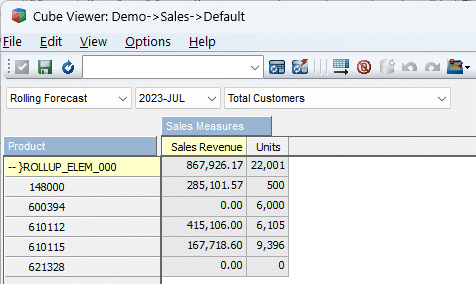
In the above snip, the result of selecting the 4 members and then rolling them up shows as a custom rollup denoted by the }ROLLUP_ELEM_xxx name.

This functionality would essentially give you the sum of the values in the columns across the members on the row.

With MDX you can achieve the same result as the above but you have many more functions and flexibility when applying these to your sets.

To get a total of the numeric values like in the cube view above, you could use the Sum() or Aggregate() functions. Both will do the same in this example.

Sum() is typically faster on basic sets requiring numeric aggregation

Aggregate() respects the cube’s default aggregation function, which may be sum, average, min, max, etc., depending on the measure’s definition. Would need to research more on this for TM1/Planning Analytics to see where any differences between the two functions come into play with our cubes.

Both functions have an optional expression that can be supplied to modify the values being aggregated.

As an example, you may give a 10% discount on all orders greater than a certain value e.g. 200,000. Aggregate() allows you to derive this 10% discount given the right case and then show the total discount.

The SUM() function

Let’s look at using the Sum() funtion first as applying this is fairly simple.

				
					SUM(Set_Expression [ , Numeric_Expression ])

For the first example, we will simply perform a sum on our set to replicate the Architect view above.

I could use PAW to add this for me by right-clicking the row header and then selecting Summarize all

The result is as follows:

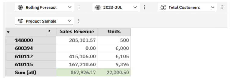
Same answer as Architect however, PAW adds in the calculated member at the bottom as a total. This can be moved to the top by updating the MDX:

				
					WITH 
	MEMBER [Product].[Product].[Sum (all)] AS 
		SUM(
		{TM1SubsetToSet([Product].[Product],"Product Sample","public")}
		), 
		SOLVE_ORDER = 1, FORMAT_STRING = '#,##0.00;(#,##0.00)' 
SELECT
NON EMPTY 
	{
		[Sales Measures].[Sales Measures].[Sales Revenue], 
		[Sales Measures].[Sales Measures].[Units]
	} ON 0, 
NON EMPTY 
	{
		{[Product].[Product].[Sum (all)]},
		{TM1SubsetToSet([Product].[Product],"Product Sample","public")}
	} ON 1 
FROM [Sales] 
WHERE (
	[Scenario].[Scenario].[Rolling Forecast], 
	[Period].[Period].[2023-JUL], 
	[Customer].[Customer].[Total Customers])

If you used PAW to create the Sum (all) calculated member, you would have noticed when you looked at the MDX that there is a lot more code than my example above. PAW adds code to remove duplicates and get a distinct set of members. This complicates our example but may be useful for later review to ensure that you understand what it is doing in case results differ to expectations.

With the updated MDX and the placement of the Sum (All) calculated member above the Product set, we mimic what we saw in Architect.

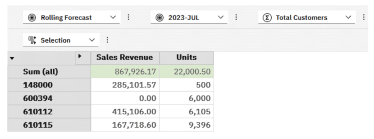
Summarize all vs Set consolidation

If you are using PAW, you would have noticed that there is another option above Summarize all called Set consolidations. As its name suggests, this will simply perform an aggregate function on the entire set rather than the Summarize all which summarizes displayed elements whether from a save set or just selected in the set editor.

Combining Arithmetic Calculations and Aggregations

If we wanted to add in the Discount at 10% where Sales Revenue is greater than 200,000, we could use the Sum() function again but add a condition to this.

				
					WITH 
	MEMBER [Product].[Product].[Sum (all)] AS 
		SUM(
		{TM1SubsetToSet([Product].[Product],"Product Sample","public")}
		), 
		SOLVE_ORDER = 1, FORMAT_STRING = '#,##0.00;(#,##0.00)' 
	MEMBER [Product].[Product].[Discount] AS 
		SUM(
		{TM1SubsetToSet([Product].[Product],"Product Sample","public")},
		CASE
			WHEN [Sales Measures].[Sales Measures].[Sales Revenue] > 200000
				THEN [Sales Measures].[Sales Measures].[Sales Revenue] * -0.1
			ELSE 0
		END
		), 
		SOLVE_ORDER = 2, FORMAT_STRING = '#,##0.00;(#,##0.00)' 
SELECT
NON EMPTY 
	{
		[Sales Measures].[Sales Measures].[Sales Revenue], 
		[Sales Measures].[Sales Measures].[Units]
	} ON 0, 
NON EMPTY 
	{
		{[Product].[Product].[Sum (all)]},
		{TM1SubsetToSet([Product].[Product],"Product Sample","public")},
		{[Product].[Product].[Discount]}
	} ON 1 
FROM [Sales] 
WHERE (
	[Scenario].[Scenario].[Rolling Forecast], 
	[Period].[Period].[2023-JUL], 
	[Customer].[Customer].[Total Customers])

				
					WITH 
	MEMBER [Period].[Period].[2023].[MAR + 6.75%] 
	AS [Period].[Period].[2023-MAR]*1.0675, 
	SOLVE_ORDER = 1, FORMAT_STRING = '#,##0.00;(#,##0.00)' 
SELECT
NON EMPTY 
	{GENERATE(
		{TM1SubsetToSet([Period].[Period],"Current Year Periods","public")}, 
		{StrToSet(
			CASE
				WHEN [Period].[Period].CURRENTMEMBER.PROPERTIES("MEMBER_NAME") = "2023-MAR" 
					THEN "{[Period].[Period].[2023-MAR], [Period].[Period].[MAR + 6.75%]}" 
				ELSE "{[Period].[Period].CURRENTMEMBER}" END
			)}
		)} ON 0, 
NON EMPTY 
  {DRILLDOWNMEMBER(
    {[Product].[Product].[Total Products]},
    {[Product].[Product].[Total Products]}
	)} ON 1 
FROM [Sales] 
WHERE ([Scenario].[Scenario].[Actual], 
	[Sales Measures].[Sales Measures].[Sales Revenue], 
	[Customer].[Customer].[Total Customers])

In the above I am using a CASE statement, more as an illustration should you need it elsewhere. An IIF() would have worked just as well in this example.

In our data we had two Products with Sales Revenue exceeding 200,000.

148000 -> 285,101.57
610112 -> 415,106.00
10% of this would be 28,510.16 and 41,510.60 respectively, giving us 70,020.76

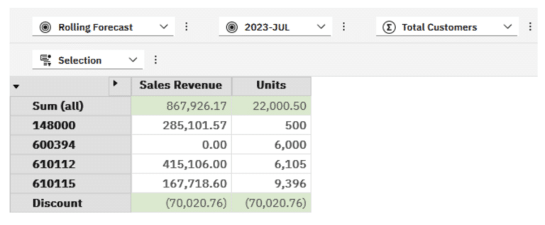
I am sure you spotted the issues with the above immediately. The Units reflects the same value in Discount and the Sum (all) does not include the Discount. Ideally we would want to see Sales Revenue net of Discount or possibly even the Sum (all) as a sub-total and then an overall total net of discount.

Let’s address the issue with the Units first. We would only want to calculate the Discount if we are dealing with the Sales Revenue measure. For anything else we would want to show a zero.

In this case, we can apply the IIF() statement before we calculate the Discount.

				
					WITH 
	MEMBER [Product].[Product].[Sum (all)] AS 
		SUM(
		{TM1SubsetToSet([Product].[Product],"Product Sample","public")}
		), 
		SOLVE_ORDER = 1, FORMAT_STRING = '#,##0.00;(#,##0.00)' 
	MEMBER [Product].[Product].[Discount] AS
		IIF(
			/* We are only interested in the Sales Revenue */
			[Sales Measures].[Sales Measures].CurrentMember.Name="Sales Revenue",
				SUM(
				{TM1SubsetToSet([Product].[Product],"Product Sample","public")},
				CASE
					/* Apply 10% to Sales Revenue over 200,000 */
					WHEN [Sales Measures].[Sales Measures].[Sales Revenue] > 200000
					THEN [Sales Measures].[Sales Measures].[Sales Revenue] * -0.1
					ELSE 0
				END)
			,0
		  ), 
		SOLVE_ORDER = 2, FORMAT_STRING = '#,##0.00;(#,##0.00)' 
SELECT
NON EMPTY 
	{
		[Sales Measures].[Sales Measures].[Sales Revenue], 
		[Sales Measures].[Sales Measures].[Units]
	} ON 0, 
NON EMPTY 
	{
		{[Product].[Product].[Sum (all)]},
		{TM1SubsetToSet([Product].[Product],"Product Sample","public")},
		{[Product].[Product].[Discount]}
	} ON 1 
FROM [Sales] 
WHERE (
	[Scenario].[Scenario].[Rolling Forecast], 
	[Period].[Period].[2023-JUL], 
	[Customer].[Customer].[Total Customers])

The above MDX now renders the following view which addresses the Units Discount issue but not the Totals.

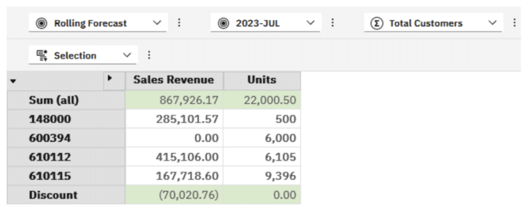
Notice too that in my MDX code I added inline comments using familiar commenting syntax /* … */

Unfortunately PAW strips these out when it processes the MDX back to the server when you click OK.

The other annoying habit PAW has is that it strips out all formatting. The indentation and line breaks are all removed returning a block of code.

I typically end up keeping my MDX code in books elsewhere for ease of update / maintenance as well as using them as a basis for future queries.

Tip:

When needing to update your MDX in the future, especially fairly lengthy code, this wall of code is not the easiest to work with and requires time to reformat. Assuming you do not have a copy of the formatted MDX saved and open a view from PAW/PAfE, you can save time and get consistent formatting by leveraging ChatGPT:

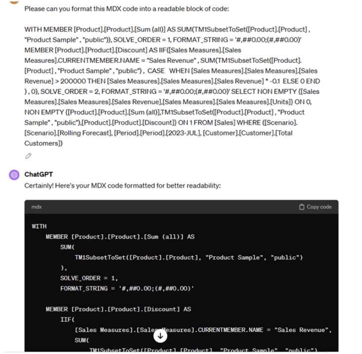
For the next part of our requirement, let’s assume that we want to show a Total, Sub-total before Discount and the Discount amount. We would need to update our MDX to include the additional calculated member and then rename Sum (all) to something more relevant.

We may also need to order these totals more logically e.g.

Product Sales Revenue on rows, then

Sub-Total,

Discount

Net Sales Revenue

We would need to rename our calculated members, add a new calculated member for the Net Sales Revenue, reorder the members displayed on the rows and also limit the display to the Sales Revenue column for now as we do not want to show values under units.

The updated MDX code would be something like the below:

				
					WITH 
	MEMBER [Product].[Product].[Sub-Total] AS 
		SUM(
			{TM1SubsetToSet([Product].[Product],"Product Sample","public")}
		 ), 
		SOLVE_ORDER = 1, FORMAT_STRING = '#,##0.00;(#,##0.00)' 
	MEMBER [Product].[Product].[Discount] AS
		IIF(
			/* We are only interested in the Sales Revenue */
			[Sales Measures].[Sales Measures].CurrentMember.Name="Sales Revenue",
				SUM(
				{TM1SubsetToSet([Product].[Product],"Product Sample","public")},
				CASE
					/* Apply 10% to Sales Revenue over 200,000 */
					WHEN [Sales Measures].[Sales Measures].[Sales Revenue] > 200000
					THEN [Sales Measures].[Sales Measures].[Sales Revenue] * -0.1
					ELSE 0
				END)
			,0
			), 
		SOLVE_ORDER = 2, FORMAT_STRING = '#,##0.00;(#,##0.00)'
	MEMBER [Product].[Product].[Net Sales Revenue] AS 
		IIF(
			/* We are only interested in the Sales Revenue */
			[Sales Measures].[Sales Measures].CurrentMember.Name="Sales Revenue",
				[Product].[Product].[Sub-Total] + [Product].[Product].[Discount], 
				0
			),
		SOLVE_ORDER = 3, FORMAT_STRING = '#,##0.00;(#,##0.00)' 		
SELECT
NON EMPTY 
	{
		[Sales Measures].[Sales Measures].[Sales Revenue], 
		[Sales Measures].[Sales Measures].[Units]
	} ON 0, 
NON EMPTY 
	{
		{TM1SubsetToSet([Product].[Product],"Product Sample","public")},
		{[Product].[Product].[Sub-Total]},
		{[Product].[Product].[Discount]},
		{[Product].[Product].[Net Sales Revenue]}
	} ON 1 
FROM [Sales] 
WHERE (
	[Scenario].[Scenario].[Rolling Forecast], 
	[Period].[Period].[2023-JUL], 
	[Customer].[Customer].[Total Customers])

The AGGREGATE() function

Without having the ability to flag measures as non-additive in TM1 so that MDX would treat them differently when aggregating, I do not have any relevant examples to share.

To date, all my testing seems to show the same values as using the Sum() function.

If anyone comes across some examples where their results differ, would be good to hear about them so that they can enhance this article.

Other Aggregation Functions

The AVG() function

The AVG() or Average function can be useful when looking at high-level information e.g. Average Sales Revenue per month.

				
					WITH 
	MEMBER [Period].[Period].[Average] AS 
	AVG(
		{TM1SubsetToSet([Period].[Period],"All Periods","public")}
	), 
	SOLVE_ORDER = 1, FORMAT_STRING = '#,##0.00;(#,##0.00)' 
SELECT 
	NON EMPTY {[Product].[Product].[Total Products]} ON 0,
	NON EMPTY {{TM1SubsetToSet([Period].[Period],"All Periods","public")}, {[Period].[Period].[Average]}} ON 1	
FROM [Sales]
WHERE ([Scenario].[Scenario].[Rolling Forecast], 
	[Sales Measures].[Sales Measures].[Sales Revenue], 
	[Customer].[Customer].[Total Customers])

The MDX code above gives us the following view:

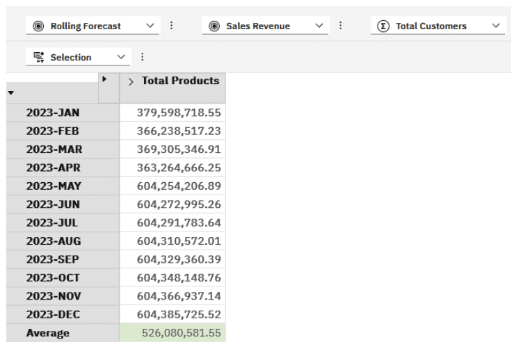
I may want to add in a Rolling Average column to show the average of the months, based on prior months.

There are a couple of considerations on this:

We will use the PeriodsToDate() function on the Period dimension. Essentially we will look at a level in which the month falls like Years to get the siblings of the current period. In our case when looking at our 2023 data, the parent is 2023 and is at level0000.

I have named my hierarchy in the }HierarchyProperties cube per the below:

Don’t forget to run a RefreshMdxHierarchy( ‘Period’ ); via TI to update any changed names.

Assuming we use some MDX code like:

				
					PERIODSTODATE([Period].[Period].[Years] , [Period].[Period].[2023-MAR])

I would expect to get 2023-JAN, 2023-FEB, 2023-MAR as members per below:

We now have a way to get the periods needed for each month.

Next we would need to add another calculated member for our Rolling Average then show it next to the monthly value for Total Products i.e. this calculated measure is defined on the Product dimension, not Period.

We could then build our MDX per the below:

				
					WITH 
	MEMBER [Period].[Period].[Average] AS 
	AVG(
		{TM1SubsetToSet([Period].[Period],"All Periods","public")}
	), 
	SOLVE_ORDER = 2, FORMAT_STRING = '#,##0.00;(#,##0.00)' 
	MEMBER [Product].[Product].[YTD Average] AS
		AVG(
			PeriodsToDate([Period].[Period].[Years], [Period].[Period].CURRENTMEMBER),
			[Product].[Product].[Total Products]),
	SOLVE_ORDER = 1, FORMAT_STRING = '#,##0.00;(#,##0.00)' 
SELECT 
	NON EMPTY {[Product].[Product].[Total Products], [Product].[Product].[YTD Average]} ON 0,
	NON EMPTY {{TM1SubsetToSet([Period].[Period],"All Periods","public")}, {[Period].[Period].[Average]}} ON 1	
FROM [Sales]
WHERE ([Scenario].[Scenario].[YTD Forecast], 
	[Sales Measures].[Sales Measures].[Sales Revenue], 
	[Customer].[Customer].[Total Customers])

This should render to give us a view as follows:

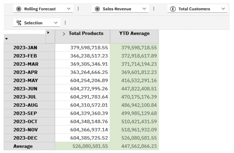
You will also notice that I needed to switch the Solve Order otherwise the Average is calculating only based on the last month.

Similarly, we could introduce the SUM() function again to give us a cumulative total:

				
					WITH 
	MEMBER [Period].[Period].[Average] AS 
	IIF(
		[Product].[Product].CurrentMember.Name="Total Products",
		AVG(
			  {TM1SubsetToSet([Period].[Period],"All Periods","public")}
			)
		,0), 
	SOLVE_ORDER = 3, FORMAT_STRING = '#,##0.00;(#,##0.00)' 
	MEMBER [Product].[Product].[YTD Average] AS
		AVG(
			PeriodsToDate([Period].[Period].[Years], [Period].[Period].CURRENTMEMBER),
			[Product].[Product].[Total Products]),
	SOLVE_ORDER = 1, FORMAT_STRING = '#,##0.00;(#,##0.00)' 
	MEMBER [Product].[Product].[YTD] AS
		SUM(
			PeriodsToDate([Period].[Period].[Years], [Period].[Period].CURRENTMEMBER),
			[Product].[Product].[Total Products]),
	SOLVE_ORDER = 2, FORMAT_STRING = '#,##0.00;(#,##0.00)' 
SELECT 
	NON EMPTY {[Product].[Product].[Total Products], [Product].[Product].[YTD], [Product].[Product].[YTD Average]} ON 0,
	NON EMPTY {{TM1SubsetToSet([Period].[Period],"All Periods","public")}, {[Period].[Period].[Average]}} ON 1	
FROM [Sales]
WHERE ([Scenario].[Scenario].[Rolling Forecast], 
	[Sales Measures].[Sales Measures].[Sales Revenue], 
	[Customer].[Customer].[Total Customers])

The view including the cumulative total should render as follows:

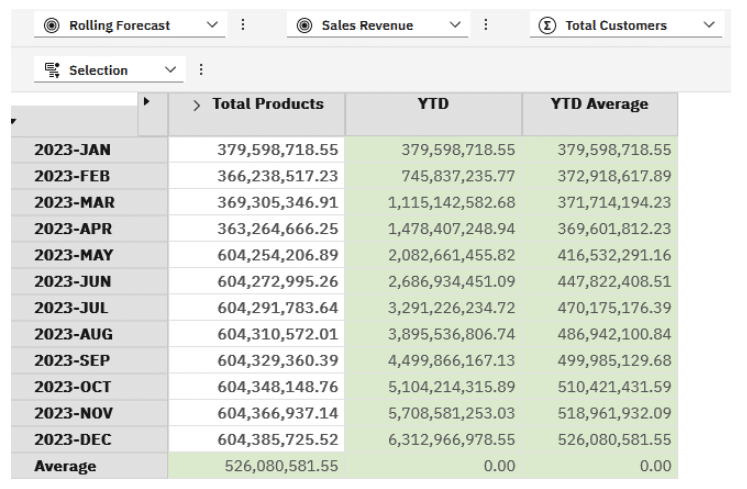
I also added an IIF() around the average as it may not make sense showing averages of YTD and YTD Average.

We have not looked at MIN() and MAX(). Most people would probably use TopCount() and BottomCount() or TopPercent() and BottomPercent() to return a list of Products or Customers as top performers or bottom performers. This is useful for analysis but you may want to look at values at a higher level in conjunction with other dimensions.

We will extend our example above to show the lowest value for each month across all Products and another column showing the highest value for each month.

The MIN() function

This function returns the minimum value for the given numeric expression, over the specified set.

We could use this to find the lowest performer based on Sales Revenue for example. We possibly need to add some additional logic to filter the values on zero Sales Revenue to avoid showing zero as the lowest value.

The MAX() function

This function returns the minimum value for the given numeric expression, over the specified set.

We could use this function to find the Sales Revenue generated by the top Customer.

The MEDIAN() function

This function will return the value of the middle most number in a set. If we were looking at Product sales across 51 items, the median would be based on the value for item 26 e.g. the Sales Revenue for item 26 when sorted. I used an odd number of elements here to keep it simple but when using a set with an even number, the median would be the average of the two middlemost element’s values.

Median may be useful in trend analysis and segmentation when looking at values for customers or products and their distance from the median. Standard deviation may also be added to this view to highlight outliers.

The STDEV() function

Standard deviation is typically used to get an idea of how widely dispersed or tightly clustered values are. Customer pricing may differ due to pricing policies applied to buying groups, volume discounts etc. Using STDEV() across a view of Customers will give insight into the sparsity or density around the mean. A wide STDEV() result may indicate very disparate pricing policies or when viewed across time, an indication of seasonality impacts.

Another example where this may be used is in manpower models when analysing a view of remuneration to get an idea of fairness around equal pay for equal work.

The VAR() function

This is not simply the difference between two members e.g. a month on month variance but rather a statistical function giving a view of the dispersion from the mean or average. This function uses the square differences from the mean to give a view of variability or consistency e.g. on the pricing across customers.

Bringing it all together

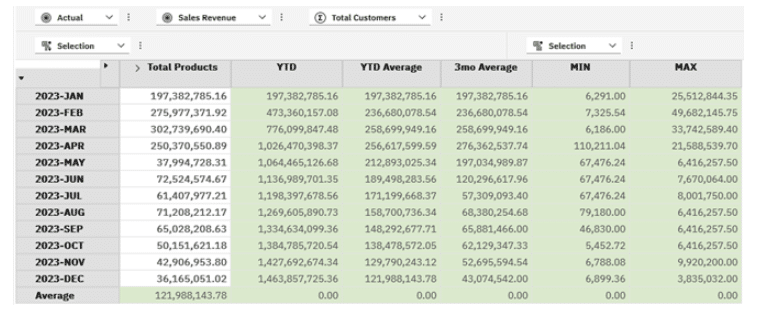
In this last example I bring a few of the functions together in a single view allowing us to see Sales Revenue for the month, a cumulative YTD view, a YTD Average, a 3 month Rolling Average, the Minimum Sales Revenue for a Product and the Maximum Sales Revenue the for the Product.

				
					WITH 
	MEMBER [Period].[Period].[Average] AS 
	IIF(
		[Product].[Product].CurrentMember.Name="Total Products",
		AVG(
			  {TM1SubsetToSet([Period].[Period],"All Periods","public")}
			)
		,0), 
	SOLVE_ORDER = 6, FORMAT_STRING = '#,##0.00;(#,##0.00)' 
	MEMBER [Product].[Product].[YTD Average] AS
		AVG(
			PeriodsToDate([Period].[Period].[Years], [Period].[Period].CURRENTMEMBER),
			[Product].[Product].[Total Products]),
	SOLVE_ORDER = 1, FORMAT_STRING = '#,##0.00;(#,##0.00)'
	
	MEMBER [Product].[Product].[YTD] AS
		SUM(
			PeriodsToDate([Period].[Period].[Years], [Period].[Period].CURRENTMEMBER),
			[Product].[Product].[Total Products]),
	SOLVE_ORDER = 2, FORMAT_STRING = '#,##0.00;(#,##0.00)'
	
	MEMBER [Product].[Product].[MIN] AS
		MIN(
			FILTER(
				{TM1FILTERBYLEVEL(TM1SUBSETALL([Product].[Product]) , 0)},
				[Sales].([Scenario].[Scenario].CurrentMember,
					[Period].[Period].CurrentMember,
					[Customer].[Customer].CurrentMember,
					[Product].[Product].CurrentMember,
					[Sales Measures].[Sales Measures].[Sales Revenue])>1
					),
			[Sales Measures].[Sales Measures].[Sales Revenue]
		),
	SOLVE_ORDER = 3, FORMAT_STRING = '#,##0.00;(#,##0.00)'
	
	MEMBER [Product].[Product].[MAX] AS
		MAX(
			{TM1FILTERBYLEVEL(TM1SUBSETALL([Product].[Product]) , 0)},
			[Sales Measures].[Sales Measures].[Sales Revenue]
		),
	SOLVE_ORDER = 4, FORMAT_STRING = '#,##0.00;(#,##0.00)'
	
	MEMBER [Product].[Product].[3mo Average] AS
		AVG(
			LastPeriods(3, [Period].[Period].CURRENTMEMBER),
			[Product].[Product].[Total Products]
		),
	SOLVE_ORDER = 5, FORMAT_STRING = '#,##0.00;(#,##0.00)'

SELECT 
	NON EMPTY {[Product].[Product].[Total Products], 
		[Product].[Product].[YTD], 
		[Product].[Product].[YTD Average],
		[Product].[Product].[3mo Average],
		[Product].[Product].[MIN],
		[Product].[Product].[MAX]} ON 0,
	NON EMPTY {{TM1SubsetToSet([Period].[Period],"All Periods","public")}, {[Period].[Period].[Average]}} ON 1	
FROM [Sales]
WHERE ([Scenario].[Scenario].[Actual], 
	[Sales Measures].[Sales Measures].[Sales Revenue], 
	[Customer].[Customer].[Total Customers])

A couple of things to note in the code above:

I switched to Actuals from Rolling Forecast as I have more variability on the data here and can better illustrate the concepts.
The MIN() function is applied to a set where I have filtered out Sales Revenue less than 1. This will remove zeroes and trivial values.
On the 3 month Average I am using the LastPeriods() function to give me the Periods I need.

The view returned is per below:

Periodic Comparisons

Another often required view is one where the user is presented with values from the current Period, prior Period, YTD and Prior Year.

This can be achieved through calculated members users some of what we have learned above.

				
					WITH 
    MEMBER [Sales Measures].[Prior Month] AS 
        (
			[Period].[Period].CurrentMember.Lag(1),
        	[Sales Measures].[Sales Revenue]            
        ), 
        SOLVE_ORDER = 1, 
        FORMAT_STRING = '#,##0.00;(#,##0.00)'
        
    MEMBER [Sales Measures].[YTD] AS 
        SUM(
			PeriodsToDate([Period].[Period].[Years], [Period].[Period].CurrentMember),
			[Sales Measures].[Sales Revenue]            
        ), 
        SOLVE_ORDER = 2, 
        FORMAT_STRING = '#,##0.00;(#,##0.00)'
	MEMBER [Sales Measures].[Prior Year] AS 
        (
			[Period].[Period].CurrentMember.Lag(12),
            [Sales Measures].[Sales Revenue]            
        ), 
        SOLVE_ORDER = 1, 
        FORMAT_STRING = '#,##0.00;(#,##0.00)'
SELECT 
    NON EMPTY {
        [Sales Measures].[Sales Revenue],
        [Sales Measures].[Prior Month],
        [Sales Measures].[YTD],
		[Sales Measures].[Prior Year]
    } ON 0,
    
    NON EMPTY TM1SubsetToSet([Product].[Product], "Default", "public") ON 1 
    
FROM [Sales]
WHERE (
    [Scenario].[Scenario].[Actual], 
    [Period].[Period].[2023-JUL], 
    [Customer].[Customer].[Total Customers])

I am using PeriodsToDate again to give us the YTD view. For Prior Month and Prior Year, I am using the Lag() function to navigate to prior Periods based on the CurrentMember.
For Prior Month, there is a lag of 1 and for Prior Year, there is a lag of 12 periods. Note that in my model 2023-JAN is the first month. If I had selected my Period as 2023-JAN, both Prior Month and Prior Year would show the same value being that of 2023-JAN as we cannot navigate to a member before the first one.

This could lead to confusion in models with insufficient history where the first month’s value may be shown.

The code above returned the view below which gives us our current Period’s Sales Revenue and the comparatives in the calculated members.

Summary

In this part we looked at some of the Aggregate functions and some applications of these. These can be valuable in giving the reader additional information they may need otherwise have had to export to Excel and added the logic there or a developer would have needed to build rules into the TM1 model for these.

There are pros and cons with building these into TM1, even if you use feederless C-level rules.

My argument is typically that these Aggregate functions have quite specific use cases and are looked at from a high-level. Creating these rules could be tricky and add a lot more overhead to the performance of the model.

Additionally, a rule to create a 3 month rolling average typically requires you to have rollups of the periods so that you can use the aggregate value to divide and get to an average. That requires additional members, maintenance and complexity. MDX is certainly easier.

Likewise with a cumulative value over time, YTD values are added as consolidations with the necessary children. Nothing wrong with this but requires additional maintenance. In the example above, if we were using C levels for the YTD members, we could not get a view with the cumulative total as presented as the Period is on rows.

Using a traditional approach would require use to have months and YTD members on the rows adding noise to the view.

Similarly, creating a native view to show the current Period, Prior Month, YTD and Prior Year is possible using MDX on the periods and putting Period on the columns but you lose the ability to change the Period and update the view based on the new selection as the MDX would need to be based on a set. You may be able to get around this by using a user preferences cube with a picklist on a measure for period and incorporating that into your Period MDX but you will be jumping through a few more hoops to get this working.

MDX views are clearly powerful tools in the modeler’s toolbox giving the modeler the ability to cater to many analysis and reporting requirements, even where the underlying fields are not present in the model but can be derived from the data and master data.

As always, please give me some feedback if I have made any errors, you have something to add etc.

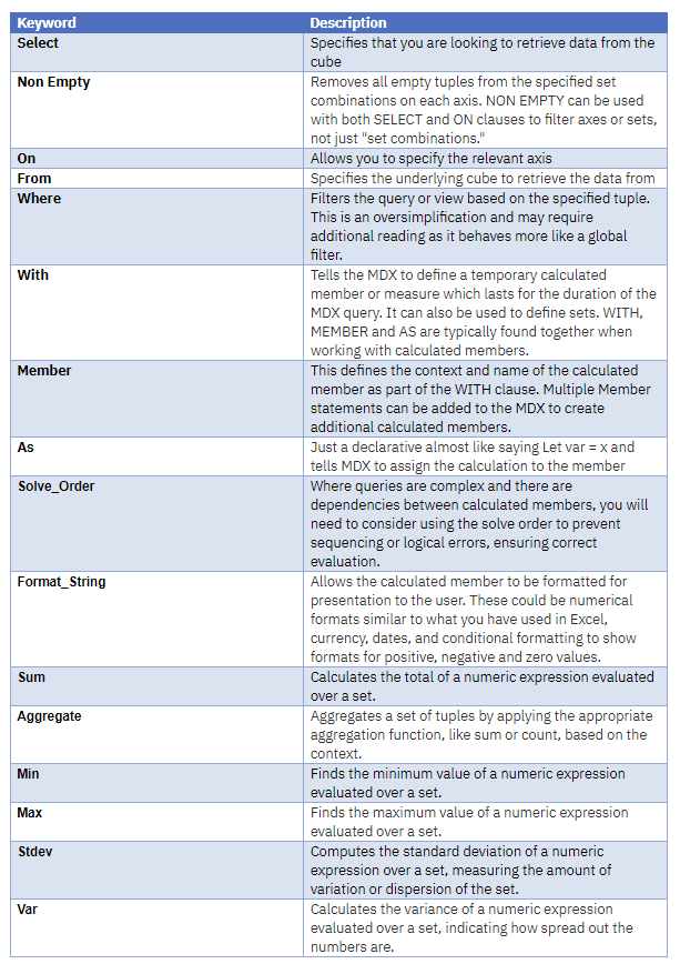
A summary of the MDX view related keywords used up to now:

By George Tonkin, Business Partner at MCi.

2 Responses

Pingback: Working with Time Series in MDX Views - Part 6 - MCi
Pingback: Untangle your Planning Analytics model string by string - MCi

Aggregate Calculated Members in MDX

The SUM() function

Summarize all vs Set consolidation

Combining Arithmetic Calculations and Aggregations

Tip:

The AGGREGATE() function

Other Aggregation Functions

The AVG() function

The MIN() function

The MAX() function

The MEDIAN() function

The STDEV() function

The VAR() function

Bringing it all together

Periodic Comparisons

Summary

Further Reading

2 Responses

Address

Ground Floor, Office 1
18 Nicol Road
Bedfordview
Johannesburg, 2007

Sign up to our Newsletter

Aggregate Calculated Members in MDX

The SUM() function

Summarize all vs Set consolidation

Combining Arithmetic Calculations and Aggregations

Tip:

The AGGREGATE() function

Other Aggregation Functions

The AVG() function

The MIN() function

The MAX() function

The MEDIAN() function

The STDEV() function

The VAR() function

Bringing it all together

Periodic Comparisons

Summary

Further Reading

2 Responses

Address

Ground Floor, Office 1 18 Nicol Road Bedfordview Johannesburg, 2007

Sign up to our Newsletter

Ground Floor, Office 1
18 Nicol Road
Bedfordview
Johannesburg, 2007