Joining Related Cube Data

Introduction

In many cases there is a need to look at related values between cubes. A basic example may be where you have product pricing in one cube and your final sales plan with your sales revenue and average price in another. Other examples include allocation models where you need to compare the base value before allocation and the ratios which may reside in separate cubes, and the results after allocation to ensure that the before and after values are the same.

Using a spreadsheet example with PAfE custom or dynamic reports makes it fairly easy to combine values from the two cubes where they share commonality e.g. on the Product dimension. DBR/W formulas to read from the sales plan can drive the report. A separate column to read from the sales price cube could be used to pull in the sales price for each product and a formula added to show any variances.

In PAW what you typically find is that the report author has created a canvas with two widgets, one for the sales plan and another with the sales price. Synchronisation and using gestures are configured to facilitate better navigation. Sometimes the report author has included a drill-through view as an alternative to cater to other shortcomings.

But what if you could just add extra columns into a PAW view like you can in a custom or dynamic report?

Well, you can and this article will describe how you can join, stitch or zip multiple cubes together to give one view with the insights you need!

Linking to the Attributes Cube

Our first example will look at including an attribute from the Product attributes. And yes, you can add attributes to the rows or columns by selecting these in PAW but what I am looking for is including the attributes in the data area so that I can use the values to drive some formatting.

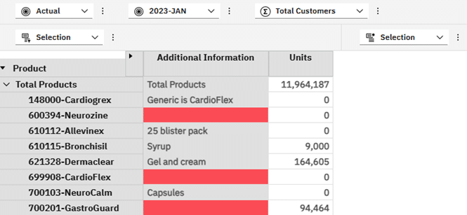
Let’s start with a basic cube view like the one below where I have included the Additional Information as an attribute to show the difference between this and adding it into the data area.

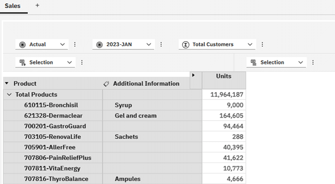
The syntax for my view shown above is:

				
					SELECT NON EMPTY 
   { [Sales Measures].[Sales Measures].[Units] } ON 0, NON EMPTY 
   { Descendants(
       TM1SubsetToSet([Product].[Product], "Default", "public") ) } ON 1 
FROM
   [Sales] 
WHERE (
   [Scenario].[Scenario].[Actual], 
   [Period].[Period].[2023-JAN], 
   [Customer].[Customer].[Total Customers])

As you can see from the code above, the Additional Information attribute is handled by the PAW interface, not through MDX.

Let’s add the Additional Information attribute as a calculated member and include it to the left of Units.

The basic syntax that we will need to refer to data in another cube (as we saw in the previous part of this series) is:

				
					[cube].(
	[dim_1].[hier_1].[member_1],
	…
	[dim_n].[hier_n].[member_n])

By specifying the cube and qualified members for each dimension, we can read a value back from the cube. The concept is very similar to how you would address a cell using a DBR/W in PAfE except that we provided the dimension and hierarchy names along with each member.

Our updated MDX would now be constructed as:

				
					WITH MEMBER [Sales Measures].[Sales Measures].[Additional Information] AS
	[}ElementAttributes_Product].(
		[Product].[Product].CurrentMember,
		[}ElementAttributes_Product].[}ElementAttributes_Product].[Additional Information])
		
SELECT NON EMPTY 
   {    [Sales Measures].[Sales Measures].[Additional Information],
		[Sales Measures].[Sales Measures].[Units] } ON 0, NON EMPTY 
   {    Descendants(
            TM1SubsetToSet([Product].[Product], "Default", "public") ) } ON 1 
FROM
   [Sales] 
WHERE (
   [Scenario].[Scenario].[Actual], 
   [Period].[Period].[2023-JAN], 
   [Customer].[Customer].[Total Customers])

If you are wondering why you would write the MDX per above to refer to attributes and not just get the values via the properties, this is purely to get the example to lead into the next section. If you were going to do the same using the properties of the Product, your MDX would simply be:

				
					WITH MEMBER [Sales Measures].[Sales Measures].[Additional Information] AS
	[Product].[Product].CurrentMember.Properties("Additional Information", TYPED)
		
SELECT NON EMPTY 
   {    [Sales Measures].[Sales Measures].[Additional Information],
		[Sales Measures].[Sales Measures].[Units] } ON 0, NON EMPTY 
   {    Descendants(
            TM1SubsetToSet([Product].[Product], "Default", "public") ) } ON 1 
FROM
   [Sales] 
WHERE (
   [Scenario].[Scenario].[Actual], 
   [Period].[Period].[2023-JAN], 
   [Customer].[Customer].[Total Customers])

Sticking with our example, the MDX using the attributes cube reference returned the following view:

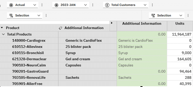
For the most part this looks good except for the 0.00 where the value of the Additional Information attribute in the attributes cube is blank.

Let’s fix that by applying some logic to check if we have a blank and should highlight this to the user where the Product is at a leaf level.

				
					WITH 
   MEMBER [Sales Measures].[Sales Measures].[Additional Information Attribute_}QSM] AS
	[}ElementAttributes_Product].(
		[Product].[Product].CurrentMember,
		[}ElementAttributes_Product].[}ElementAttributes_Product].[Additional Information])

   MEMBER [Sales Measures].[Sales Measures].[Additional Information] AS
	IIF( IsLeaf([Product].[Product].CURRENTMEMBER),
         IIF( [Sales Measures].[Sales Measures].[Additional Information Attribute_}QSM] = 0,
            "",
            [Sales Measures].[Sales Measures].[Additional Information Attribute_}QSM]),
       [Product].[Product].CurrentMember.Name)

SELECT NON EMPTY 
   {    [Sales Measures].[Sales Measures].[Additional Information],
		[Sales Measures].[Sales Measures].[Units] } ON 0, NON EMPTY 
   {    Descendants(
            TM1SubsetToSet([Product].[Product], "Default", "public") ) } ON 1 
FROM
   [Sales] 
WHERE (
   [Scenario].[Scenario].[Actual], 
   [Period].[Period].[2023-JAN], 
   [Customer].[Customer].[Total Customers])

First we derive the value of the attribute into a temporary variable: [Sales Measures].[Sales Measures].[Additional Information Attribute_}QSM].

I am using the “_}QSM” suffix on the end of the calculated member to indicate that this is a Query Scoped Member and would not be something needed as a member to view on rows or columns. As such, it does not appear in the Set Editor.

Using this temporary variable, I can apply my logic and derive the values needed.

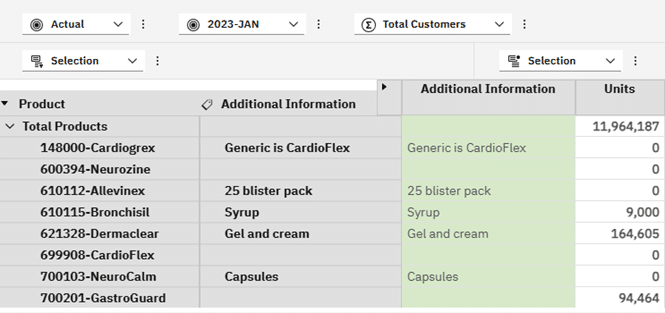
The updated view has the 0.00 removed:

As a further example of how deriving the Additional Information as data rather than attribute information added by PAW gives advantages, we can use the new Format Manager to format our cells and add some highlighting to the missing attribute values:

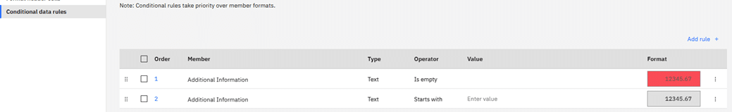
Where the attribute value is missing I want to highlight the cell in red, otherwise show it in grey like the attribute when added directly through PAW.

After hiding the attribute I added through PAW, my view now looks as follows:

Just like Additional Information which was originally shaded in green by default to show it is a calculated value, other calculated values could similarly be formatted.

Another useful feature of calculated members is that we can derive a member and give it another name e.g. Additional Information may have been derived purely as Comment. Keep in mind too that if we had derived a calculated member based on an existing measure e.g. Units, we make it a read-only value in the view and it is protected from any changes that users with permissions could inadvertently make.

Maybe not the most exciting example but keep in mind that the concepts can be used over and over again in many cases. Also keep in mind that when needing to display string values from a cube, this approach would work nicely where I could address leaf level information but show in a view that may contain consolidated members.

Linking to the Sales Price cube

My Sales model has some additional cube linkages to pricing, Customer related discounts as well as the standard or unit cost for each Product.

A simple view of sales revenue and cost of sales can be seen in the below view:

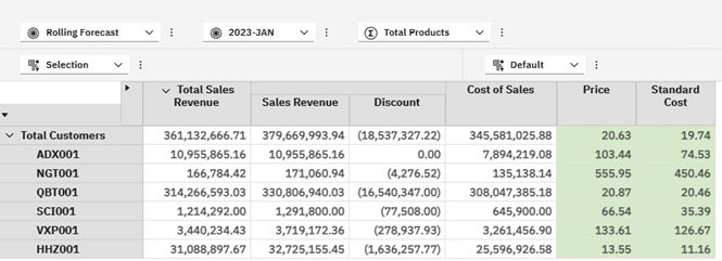
Sales Revenue is simply Units x Price (prices come from the Sales Price cube). Discount is based on a percentage agreed for each Customer.

The Cost of Sales measure is Units x Standard Cost which is constant for Customers but would vary based on the Product.

Price is an average selling price derived via rules, as Total Sales Revenue divided by Units. We divide using the \ character to avoid visible errors because of dividing by 0.

Standard Cost is simply reflecting the value from the underlying Sales Cost cube.

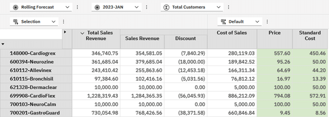
What we need to be able to see is how much on average we are discounting Products by. We will pivot the view and put Products on rows then add a look up to the Sales Price cube and show a Price Variance per line item. I am removing Total Products as an overall average Sales Price across all Products and Customers is not useful in the examples we will look at.

Our starting view is thus something like the below – remember that Price and Standard Cost are rule derived in the cube rules:

The Sales Price cube looks as follows:

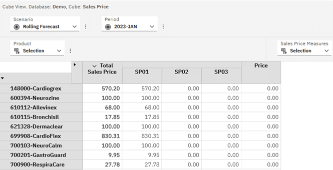
What we want to do is read the Total Sales Price for each Product based on the current Scenario and Period back into our Sales view and then use this in the variance calculation.

Our Sales Price cube has the following structure:

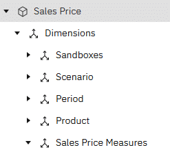
We can ignore the Sandboxes dimension in our MDX and just reference Scenario, Period, Product and the measure we need i.e. Total Sales Price, and we can call it Gross Price.

Once we have derived the Gross Price, we can create another measure called Price Variance which will simply be the difference between the Gross Price and the average Price which is rule derived in the Sales cube.

The updated MDX code is as follows:

				
					WITH 
   MEMBER [Sales Measures].[Sales Measures].[Gross Price] AS 
    [Sales Price].(
      [Scenario].[Scenario].CURRENTMEMBER,
      [Period].[Period].CURRENTMEMBER,
      [Product].[Product].CURRENTMEMBER,
      [Total Sales Price]),
      SOLVE_ORDER = 1, FORMAT_STRING = '#,##0.00;(#,##0.00)' 

   MEMBER [Sales Measures].[Sales Measures].[Price Variance] AS 
      [Sales Measures].[Sales Measures].[Gross Price] - 
      [Sales Measures].[Sales Measures].[Price], 
      SOLVE_ORDER = 2, FORMAT_STRING = '#,##0.00;(#,##0.00)'

SELECT NON EMPTY 
   {
      [Sales Measures].[Sales Measures].[Total Sales Revenue],
      [Sales Measures].[Sales Measures].[Sales Revenue],
      [Sales Measures].[Sales Measures].[Discount],
      [Sales Measures].[Sales Measures].[Cost of Sales],
      [Sales Measures].[Sales Measures].[Gross Price],
      [Sales Measures].[Sales Measures].[Price],
      [Sales Measures].[Sales Measures].[Price Variance],
      [Sales Measures].[Sales Measures].[Standard Cost]
   } ON 0, NON EMPTY 
   {
      [Product].[Product].[Total Products].CHILDREN
   } ON 1 
FROM
   [Sales] 
WHERE (
   [Scenario].[Scenario].[Rolling Forecast], 
   [Period].[Period].[2023^2023-JAN], 
   [Customer].[Customer].[Total Customers])

You will notice that the syntax we followed is identical to the previous attribute example i.e.

				
					[cube].(
	[dim_1].[hier_1].[member_1],
	…
	[dim_n].[hier_n].[member_n])

This holds true for all references used with this method of linking to other cubes, whether a model cube or control cube.

On a quick detour, there is also another function to link to other cubes called LookupCube. This works in a similar manner and has the following syntax:

				
					LookupCube("cube","([dim_1].[hier_1].[member_1], …, [dim_n].[hier_n].[member_n])")

The cube name is in the first parameter and the address reference in the next parameter. When using LookupCube, ensure that the whole function is on a single line without any breaks. Any line breaks prevent the MDX from executing as expected.

With the code above referencing the Sales Price cube and doing the difference between the Gross Price and Price we have our view as follows:

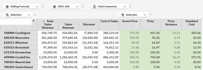
In the above, we can clearly see where the Discount has created a Price Variance. Remember that Price is rule derived and is an average for the Product across all Customers, taking their aggregate discounts into account.

We could add a Price Variance % but will leave this as an exercise for the reader. Similarly, you could add another Gross Price member and use the LookupCube function to derive the value.

Summary

This article showed two examples of reading values from another cube. Even though only one linkage was included, there is no limit to including multiple values from multiple cubes. As long as you can define the reference to the external cube, you can reference a value and show it in your view.

Sometimes like with the attribute example, you may want to include a column or row purely to drive some conditional formatting or show a variance or variance percentage. Using the concepts described above will set you up to achieve this.

In the next part, we will look at further examples of joining data from multiple cubes where dimensionality is similar but where we may need to convert measures to match the external or lookup cube.

A summary of the MDX view related keywords used up to now:

Keyword	Description
Select	Specifies that you are looking to retrieve data from the cube
Non Empty	Removes all empty tuples from the specified set combinations on each axis. NON EMPTY can be used with both SELECT and ON clauses to filter axes or sets, not just “set combinations.”
On	Allows you to specify the relevant axis
From	Specifies the underlying cube to retrieve the data from
Where	Filters the query or view based on the specified tuple. This is an oversimplification and may require additional reading as it behaves more like a global filter.
With	Tells the MDX to define a temporary calculated member or measure which lasts for the duration of the MDX query. It can also be used to define sets. WITH, MEMBER and AS are typically found together when working with calculated members.
Member	This defines the context and name of the calculated member as part of the WITH clause. Multiple Member statements can be added to the MDX to create additional calculated members.
As	Just a declarative almost like saying Let var = x and tells MDX to assign the calculation to the member
Solve_Order	Where queries are complex and there are dependencies between calculated members, you will need to consider using the solve order to prevent sequencing or logical errors, ensuring correct evaluation.
Format_String	Allows the calculated member to be formatted for presentation to the user. These could be numerical formats similar to what you have used in Excel, currency, dates, and conditional formatting to show formats for positive, negative and zero values.
Sum	Calculates the total of a numeric expression evaluated over a set.
Aggregate	Aggregates a set of tuples by applying the appropriate aggregation function, like sum or count, based on the context.
Min	Finds the minimum value of a numeric expression evaluated over a set.
Max	Finds the maximum value of a numeric expression evaluated over a set.
Stdev	Computes the standard deviation of a numeric expression over a set, measuring the amount of variation or dispersion of the set.
Var	Calculates the variance of a numeric expression evaluated over a set, indicating how spread out the numbers are.
IIF()	The Immediate IF statement allows us to evaluate an expression for a certain condition and then return a result if true and a different result if false.
Case, When, Else, End	The Case statement would be used where you expect multiple outcomes or need to extend the conditions beyond true and false. The first WHEN statement that returns true is returned as the result. An ELSE can be used for a catch-all scenario or default result.
.CurrentMember	Allows us to address the current member the view is dealing with from the context area or another axis.
.Properties(“<propertyname>”<, TYPED>)	Allows us to retrieve a property value which may be an intrinsic like the Element_Level or custom like an attribute that a modeller added. Using TYPED ensures that a data type relating to the underlying definition is returned.
Instr()	Returns the position of a substring within a string, similar to TI’s Scan()
Len()	Returns the length of a string
Left()	Returns the n number of characters from the start of a string
Right()	Returns the n number of characters from the end of a string
LCase()	Returns the lower case of a string
UCase()	Return the upper case of a string
ParallelPeriod()	Returns a member from a prior period in the same relative position within a parallel period e.g. same month, last year.
LastPeriods()	Returns a set of members starting from the specified member and going backwards through the hierarchy by a specified number of periods. If given a negative number, it moves forward through the hierarchy.
PeriodsToDate()	Returns a set of periods from the beginning of a specified level to the specified member. Typically used with year-to-date views as YTD() is not supported by TM1.
OpeningPeriod()	Returns the first member of a specified level within a specified period or its ancestor e.g. January as the first month in our year.
ClosingPeriod()	Returns the last member of a specified level within a specified period or its ancestor e.g. December as the last month in our year.
Lag()	Returns the member that is a specified number of periods before the specified member in the same level. The lag can be positive to move backwards or negative to move forwards.
Lead()	Returns the member that is a specified number of periods after the current member in the same level. Similar to Lag(), you can switch signage to move backwards but better to use Lag() and Lead() as designed for better readability.
UserName	Returns a string containing the client ID of the logged in user
StrToMember()	Converts a text string to a member in the specified dimension
TM1FilterByPattern()	Allows you to implement a wildcard search against a set of members. Don’t forget the third parameter that can specify an alias or attribute to be used to search against.
LookupCube	This function is an alternative to using the [cube].(tuple) syntax. A single line should contain the following syntax: LookupCube(“cube”,”([dim1].[hier1].[member],…, [dimn].[hiern].[member])”)

Special thanks to Wim Gielis for his review and feedback.

By George Tonkin, Business Partner at MCi.